let's build a Garbage Collector (GC) from scratch

Lets build GC from scratch in go and let how it works

Hello World!

Lately, I’ve been diving deep into understanding the Garbage Collectors .The systems that quietly manage memory behind the scenes in our code. Over the past six months, I’ve spent a good amount of time reading up on how GCs work across different programming languages, trying to understand the why and how behind them.

So I thought I’d take a shot at sharing some of the key things I’ve learned, and hopefully in a way that’s approachable and helps you build a solid foundation. As always, I’ve also put together a simplified version you can play around with:

👉 Check it out on GitHub

Let’s get into it.

---

Share for Good Karma 😇

Here is what you are going to learn today!

🗂️ Table of Contents

1. Why Do We Need Garbage Collection?
   The pitfalls of manual memory management and the case for GC.

2. Core Concepts: The Foundation of GC
   Stack vs Heap, Reachability, Roots, and Object Graphs.

3. Fundamental GC Phases & Algorithms

   • Mark-and-Sweep

   • Mark-and-Compact

   • Copying Collector (Semi-Space)

   • Generational GC

4. Advanced Concepts and Considerations

   • Stop-the-World, Incremental, and Concurrent GC

   • Parallelism and Barriers

   • GC Tuning and Implementation Details

5. Trade-offs in GC Design
   Balancing throughput, latency, memory usage, and complexity.

6. The Future of Garbage Collection
   Emerging trends: ZGC, NUMA, off-heap management, adaptive GCs.

7. Conclusion
   Key takeaways and who benefits from understanding GC.

---

1. Why Do We Need Garbage Collection? The Problem of Manual Memory Management

In languages like C or C++, developers are responsible for:

1. Allocating memory: Requesting a memory block from the operating system (e.g., using malloc or new).

2. Using memory: Storing data in the allocated block.

3. Deallocating memory: It means releasing the block back to the operating system when it's no longer needed (e.g., using free or delete).

Failure to deallocate memory leads to memory leaks, where the program continuously consumes memory without releasing it, eventually exhausting system resources. Premature deallocation, while the memory is still in use, leads to dangling pointers, which can cause unpredictable behavior, crashes, or security vulnerabilities when the program tries to access memory that has been freed or reallocated.

GC aims to solve these problems by automatically identifying and reclaiming "garbage" – memory that is no longer reachable by the application.

2. The Foundation of GC

Before diving into algorithms, let's understand some fundamental concepts:

a. The Heap and The Stack:

Most programming languages divide memory into two primary regions:

• Stack: Used for static memory allocation and execution context (function call frames). Memory is managed automatically in a LIFO (Last-In, First-Out) manner. Local variables and function parameters reside here. Allocation and deallocation are extremely fast.

• Heap: Used for dynamic memory allocation, where objects with potentially longer or unknown lifetimes are stored. This is the region GC primarily manages.

Internal flow of heap and stack

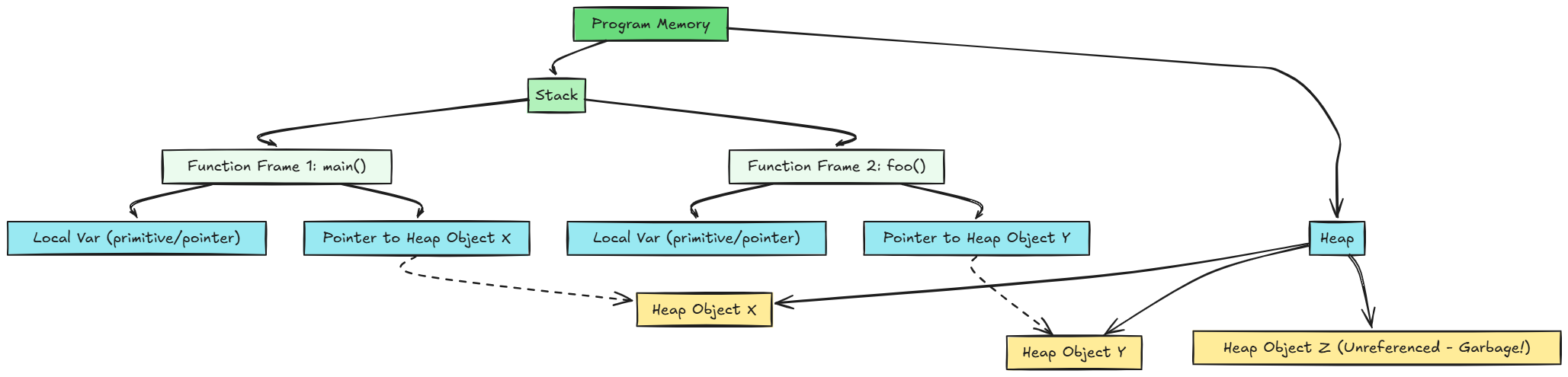
In the diagram, Object Z is on the heap but has no active pointers from the stack (or other live objects), making it garbage.

b. Reachability:

Src: Reachability

The core principle of most modern GCs is reachability. An object is considered "live" if it is reachable from a set of "root" references. If it's not reachable, it's "garbage" and can be reclaimed.

c. Roots:

Src : Garbage-collection roots

Roots are the starting points for tracing object references. They are memory locations that are inherently accessible to the program. Common examples include:

• Global variables: Variables accessible from anywhere in the program.

• Local variables and parameters on the stack: Variables within active function call frames.

• CPU registers: Pointers held directly by the CPU.

• Static variables: Variables belonging to classes rather than instances.

d. Object Graph:
Objects on the heap often reference other objects, forming a complex interconnected structure called an object graph. GC traverses this graph starting from the roots.

In this graph, Objects A, B, C, D, E, F are live. Object G and H are not reachable from any root, even if H is referenced by G.

3. Fundamental GC Phases & Algorithms

Src : Yellow are stop-the-world phases, green are concurrent phase (java)

Most GCs operate in distinct phases. While specific algorithms vary, they often involve variations of Marking, Sweeping, and/or Compacting.

a. Marking Phase:
The GC traverses the object graph, starting from the roots, to identify all reachable (live) objects.

• It typically uses graph traversal algorithms like Depth-First Search (DFS) or Breadth-First Search (BFS).

• When an object is visited, it's "marked" as live (e.g., by setting a bit in its header).

Marking (simplified DFS):

function Mark(object):
  if object is not null and object is not marked:
    mark object as live
    for each child_reference in object:
      Mark(GetObject(child_reference)) // Recursively mark children

// Main GC Mark Phase
function StartMarking():
  for each root in Roots:
    Mark(GetObject(root))

b. Sweeping Phase (for Mark-and-Sweep):
After marking, the GC scans the entire heap. Any object not marked as live is considered garbage and its memory is reclaimed.

• The reclaimed memory is typically added to a "free list" for future allocations.

• ❌This can lead to heap fragmentation, where free memory is scattered in small, non-contiguous blocks. This can make it hard to allocate larger objects even if enough total free memory exists.

c. Compaction Phase (for Mark-and-Compact):
To address fragmentation, compaction rearranges live objects in memory, moving them together into one contiguous block at one end of the heap.

• This leaves a single, large contiguous block of free memory at the other end.

• 🔻 Compaction is expensive as it involves copying objects and updating all references to them.

---

Let's look at common algorithms built upon these phases:

Algorithm 1: Mark-and-Sweep

1. Mark Phase: As described above, identify all live objects.

2. Sweep Phase: Iterate through the heap. If an object is not marked, reclaim its memory. Marked objects are unmarked for the next cycle.

Heap State Example (Mark-and-Sweep):

Initial State:
| Obj A (Live) | Obj B (Garbage) | Obj C (Live) | Free Space |

After Mark: (A and C are marked)
| Obj A (M) | Obj B | Obj C (M) | Free Space |

After Sweep:
| Obj A | ---Free (was B)--- | Obj C | Free Space |
(Note potential fragmentation between A and C)

✅Pros:

• Simple to implement.

• Handles cyclic references naturally (as long as they are not reachable from roots).

❌Cons:

• Fragmentation: Can lead to allocation failures even with sufficient total free memory.

• Stop-the-World (STW) Pauses: The entire application is typically paused during marking and sweeping. The pause time can be proportional to the heap size (for sweep) and the number of live objects (for mark).

Algorithm 2: Mark-and-Compact

1. Mark Phase: Same as Mark-and-Sweep.

2. Compact Phase: Live objects are relocated to one end of the heap. This involves:

   • Calculating new addresses for live objects.

   • Updating all pointers to these objects.

   • Moving the objects to their new addresses.

Heap State Example (Mark-and-Compact):

Initial State:
| Obj A (Live) | Obj B (Garbage) | Obj C (Live) | Free Space |

After Mark: (A and C are marked)
| Obj A (M) | Obj B | Obj C (M) | Free Space |

After Compact:
| Obj A | Obj C | -------- Large Free Space -------- |
(All pointers to A and C are updated)

✅Pros:

• No Fragmentation: Excellent for long-running applications.

• Fast allocation (just increment a pointer in the free area).

❌Cons:

• Expensive Compaction: Moving objects and updating pointers is computationally intensive.

• Longer STW Pauses: Compaction adds significant overhead to the pause.

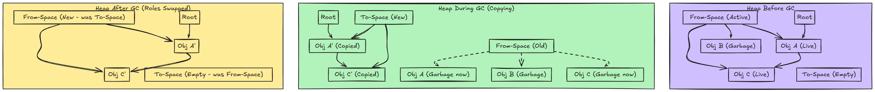
Algorithm 3: Copying Collector (Semi-Space Collector)

This algorithm divides the heap into two equal-sized semi-spaces: From-Space and To-Space.

1. All new objects are allocated in From-Space.

2. When From-Space fills up, a GC cycle begins:

   • Traverse the live objects in From-Space starting from the roots.

   • Instead of just marking, copy each live object encountered to To-Space.

   • Update pointers (from roots or already copied objects) to point to the new location in To-Space.

3. Once all live objects are copied, From-Space contains only garbage.

4. The roles of From-Space and To-Space are then swapped. The (now former) From-Space is entirely free, and To-Space becomes the new From-Space for future allocations.

Copying GC:

Heap = [FromSpace, ToSpace]
AllocationPointer = StartOf(FromSpace)

function Allocate(size):
  if AllocationPointer + size > EndOf(FromSpace):
    Collect()
  if AllocationPointer + size > EndOf(FromSpace): // Still not enough space
    throw OutOfMemoryError
  
  object_address = AllocationPointer
  AllocationPointer += size
  return object_address

function Collect():
  Swap(FromSpace, ToSpace) // ToSpace is now the new FromSpace, FromSpace is old and to be cleared
  AllocationPointer = StartOf(FromSpace) // New allocations go into the (new) FromSpace
  
  // ScanRootsAndCopy will copy reachable objects from ToSpace (old FromSpace) to FromSpace (new FromSpace)
  // and update AllocationPointer
  for each root in Roots:
    ScanRootsAndCopy(root, FromSpace, ToSpace, &AllocationPointer) // Pass AllocationPointer by reference

  Clear(ToSpace) // The old FromSpace (now ToSpace) can be cleared

function ScanRootsAndCopy(root_reference, current_from_space, current_to_space, current_alloc_ptr_ref):
  // Simplified: Imagine root_reference points to an object in current_to_space (the old FromSpace)
  object_in_old_space = GetObject(root_reference)
  
  if object_in_old_space was already copied:
    update root_reference to point to object's new_address_in_current_from_space
  else:
    new_address = *current_alloc_ptr_ref
    Copy object_in_old_space to new_address in current_from_space
    *current_alloc_ptr_ref += size_of(object_in_old_space)
    Mark object_in_old_space as copied and store its new_address (forwarding pointer)
    update root_reference to point to new_address
    
    for each child_reference in the newly copied object (in current_from_space):
      ScanRootsAndCopy(child_reference, current_from_space, current_to_space, current_alloc_ptr_ref)

Note: The actual implementation of ScanRootsAndCopy often uses Cheney's algorithm, which is a breadth-first approach and avoids deep recursion by using the To-Space itself as a queue.

Fig Copying Collector:

✅Pros:

• Fast Allocation: Allocation is just incrementing a pointer (bump allocation).

• Automatic Compaction: Live objects are naturally compacted into To-Space.

• Good for Short-Lived Objects: If many objects die quickly, From-Space clears out efficiently.

• Pause time is proportional to the number of live objects, not heap size.

❌Cons:

• Memory Overhead: Requires twice the memory (only half is usable at any time).

• Copying Cost: Copying objects can be expensive, especially for large live sets.

Algorithm 4: Generational Garbage Collection

This is one of the most impactful optimizations and is based on the Weak Generational Hypothesis:

1. Most objects die young.

2. Few objects live for a long time.

The heap is divided into (at least) two generations:

• Young Generation (Nursery): Where new objects are allocated. This space is collected frequently and usually with a copying collector (fast for mostly garbage data).

  • Often further subdivided (e.g., in Java's HotSpot VM) into:

    • Eden: New objects are allocated here.

    • Survivor Spaces (S0, S1): Objects surviving a Young GC are moved here.

• Old Generation (Tenured Generation): Objects that survive several Young GC cycles are "promoted" to the Old Generation. This space is collected less frequently, often using a Mark-and-Sweep or Mark-and-Compact algorithm because objects here are expected to live longer, making copying less efficient.

Key challenge in Generational GC: References from Old Generation objects to Young Generation objects (inter-generational pointers).

• If an Old Gen object points to a Young Gen object, that Young Gen object is live, even if no Young Gen root points to it.

• Scanning the entire Old Gen during a Young GC would defeat the purpose of fast Young GCs.

• Solution: Card Table / Remembered Set: A data structure that tracks pointers from Old Gen to Young Gen. When an Old Gen object is modified to point to a Young Gen object, this change is recorded. During a Young GC, these "dirty" cards are scanned as additional roots.

✅Pros:

• Reduced Pause Times: Frequent, short pauses for Young Gen, infrequent longer pauses for Old Gen. Overall application responsiveness improves.

• Efficiency: Different algorithms can be used for different generations, tailored to their characteristics.

❌Cons:

• Complexity: More intricate to implement and tune.

• Overhead of Remembered Sets: Maintaining card tables adds a small runtime cost (write barrier).

4. Advanced Concepts and Considerations

a. Stop-the-World (STW) Pauses:

Most traditional GCs require pausing the application threads ("stopping the world") to safely analyze and modify the heap. This ensures that the object graph doesn't change while the GC is working. Long STW pauses can severely impact application responsiveness and user experience, especially for interactive or real-time systems.

b. Incremental GC:

The GC work is interleaved with application execution. The GC performs a small amount of work, then yields to the application, then resumes.

• Goal: Reduce long STW pauses by breaking them into smaller, more frequent pauses.

• Challenge: Requires careful synchronization (e.g., read/write barriers) to handle changes made by the application while the GC is partially complete.

c. Concurrent GC:
The GC runs concurrently with application threads for significant portions of its work (e.g., marking).

• Goal: Minimize or eliminate STW pauses.

• Challenge: Highly complex. The GC must deal with an object graph that is constantly being mutated by the application. This often involves sophisticated synchronization mechanisms and re-marking phases to catch changes.

• Examples: CMS (Concurrent Mark Sweep), G1 (Garbage-First) in Java, Go's GC.

d. Parallel GC:
Uses multiple threads for GC work itself (e.g., parallel marking, parallel sweeping). This doesn't necessarily mean concurrent with the application; it often means the STW pause is shorter because the GC work is done faster by multiple CPU cores.

• Most modern GCs use parallel techniques for parts of their STW phases.

e. Read and Write Barriers:
Special instructions are inserted by the compiler at object read or write operations.

• Write Barriers: Crucial for generational GCs (updating card tables) and incremental/concurrent GCs (notifying GC about pointer modifications). For example, if objA.field = objB and objA is in Old Gen and objB is in Young Gen, a write barrier records this.

• Read Barriers: Less common, but can be used by some concurrent GCs to ensure the GC sees a consistent view of objects if an application thread reads an object while the GC is moving it.

f. GC Tuning:
Many GCs (especially in JVM, . .NET) offer a plethora of tuning options:

• Heap size (initial, maximum).

• Generation sizes and ratios.

• Choice of GC algorithm (e.g., Serial, Parallel, CMS, G1, ZGC, Shenandoah in Java).

• Pause time goals, throughput goals.

• Tuning is highly application-specific and requires understanding the application's object allocation patterns and performance requirements.

g. Specific GC Implementations :

• Java (HotSpot VM):

  • Serial GC: Single-threaded, simple, best for small applications or single-core environments.

  • Parallel GC: Multi-threaded, throughput-oriented, suitable for multi-core servers.

  • CMS (Concurrent Mark Sweep): Low-pause collector, deprecated in recent JDKs.

  • G1 GC: Default in modern JDKs, balances throughput and pause times, region-based.

  • ZGC: Scalable, low-latency, concurrent collector, suitable for large heaps.

  • Shenandoah: Low-latency, concurrent collector, similar to ZGC.

  • All are generational collectors (except ZGC/Shenandoah, which are region-based).

  ---

  .NET (CLR):

  • Generational GC: Three generations (0, 1, 2) for short-lived and long-lived objects.

  • Mark-Compact: Used for full (Gen 2) collections.

  • Workstation GC: Optimized for desktop apps, minimal pause.

  • Server GC: Optimized for throughput on multi-core servers, uses multiple threads.

  ---

  Go:

  • Concurrent, tri-color mark-and-sweep: Designed for low latency.

  • Not generational (as of now), but research is ongoing.

  • Write barriers are used to maintain correctness during concurrent marking.

  ---

  Python (CPython):

  • Reference Counting: Immediate reclamation of unreachable objects.

  • Cyclic GC: Detects and collects reference cycles not handled by reference counting.

  • Not generational in the traditional sense, but divides objects into three "generations" for cycle detection.

  ---

5. Trade-offs in GC Design

Choosing or designing a GC involves balancing several competing goals:

Throughput

• The proportion of total CPU time spent doing application work versus garbage collection.

• High throughput: Means more time is spent running user code, less on GC. Important for batch jobs, backend services.

• Example: Java’s Parallel GC is optimized for throughput, using multiple threads to minimize GC time.

---

Latency (Pause Time)

• The duration for which application threads are paused during GC.

• Low latency: Critical for interactive or real-time applications (e.g., trading systems, games).

• Concurrent GCs: (e.g., Java G1, ZGC, Shenandoah, Go’s GC) minimize pause times by performing most GC work concurrently with application threads.

• Stop-the-world (STW): GCs like Serial or Parallel GC can have longer pauses.

---

Memory Footprint

• The extra memory required by the GC for its operation (e.g., survivor spaces, mark bitmaps, card tables).

• Copying collectors: Need extra space for to-space.

• Concurrent/incremental collectors: May require additional metadata (e.g., remembered sets, write barriers).

• Trade-off: Lower memory footprint can reduce costs but may increase GC frequency.

---

Scalability

• How well the GC performs as heap size and CPU core count increase.

• Multi-threaded GCs: (e.g., Java Parallel GC, .NET Server GC) scale well with more cores.

• Large heaps: Modern GCs like G1, ZGC, and .NET’s Server GC are designed to handle large heaps efficiently.

---

Portability & Complexity

• Portability: How easily the GC can be ported to different platforms/architectures.

• Complexity: More advanced GCs (concurrent, generational, region-based) are harder to implement and maintain.

• Example: Reference counting is simple and portable, but less efficient for cycles and performance.

---

Determinism

• Predictability of GC pauses and behavior.

• Real-time GCs: Aim for predictable, bounded pause times (e.g., Azul C4, some research GCs).

• Most mainstream GCs: Offer best-effort, not strict determinism.

---

Configurability & Tuning

• Ability to tune GC parameters for specific workloads (e.g., heap size, pause goals).

• Java: Offers many GC tuning flags.

• .NET: Has configuration for workstation/server modes, latency modes.

---

Monitoring & Diagnostics

• Support for logging, metrics, and analysis of GC behavior.

• Modern runtimes: Provide detailed GC logs and metrics for troubleshooting and optimization.

---

Often, improving one aspect comes at the cost of another (e.g., reducing latency with concurrent GC might slightly reduce throughput due to barrier overhead and coordination).

6. The Future of Garbage Collection

GC is a continuously evolving field:

• Ultra-Low Latency GCs: Aiming for sub-millisecond pauses (e.g., ZGC, Shenandoah).

• NUMA-Aware GCs: Optimizing for Non-Uniform Memory Access architectures.

• Off-Heap Memory Management: More applications are using memory outside the GC's managed heap for performance-critical data structures, requiring careful manual or semi-automated management.

• Integration with Hardware: Research into hardware-assisted GC.

• Adaptive GCs: GCs that can dynamically change their strategies based on application behavior.

Conclusion

Garbage Collection is a cornerstone of modern managed programming languages, significantly boosting developer productivity and reducing common memory-related errors. From simple Mark-and-Sweep to sophisticated concurrent, generational collectors like G1 or ZGC, the field has seen immense innovation.

While GC automates much, a good understanding of its workings helps in writing memory-efficient applications and diagnosing performance issues when they arise. It remains a fascinating and active area of computer science research and engineering.

---

GC from scratch

Mark-Sweep Garbage Collector

• Generational Collection - Efficiently manages objects in young and old generations

• Concurrent Marking - Minimizes stop-the-world pauses

• Cycle Detection - Properly handles circular references

• Thread-Safe - Safe for concurrent use across goroutines

• Configurable - Tunable parameters for different workloads

• Comprehensive Metrics - Detailed statistics and monitoring

• Finalization Support - Cleanup hooks for resource management

Reference Counting Garbage Collector

• Immediate Reclamation - Objects are collected as soon as they become unreachable

• Simple Implementation - Easy to understand and reason about

• Low Pause Times - No stop-the-world pauses during collection

• Thread-Safe - Safe for concurrent use across goroutines

• Deterministic Cleanup - Finalizers run immediately when objects are collected

Please read more here : Check it out on GitHub 👈

Share for Good Karma 😇

Liked this article? Make sure to ❤️ click the like button.

Feedback or addition? Make sure to 💬 comment.

Know someone who would find this helpful? Make sure to 🔁 share this post.

Your support means a great deal!

Thank you! Let’s learn together!