Paper I read this week: BigTable

Lets understand how BigTable works

Okay, let's dive into the foundational Bigtable paper.

"Bigtable: A Distributed Storage System for Structured Data" by Fay Chang et al. from Google. This is one of those seminal papers that shifted how people thought about handling truly massive datasets. We'll try to understand by focusing on the core ideas, the engineering choices, and why it was so influential. In this article, we will review this paper, learn key insights, and discuss the distributed systems engineering part of it.

You can read the paper here as well:

https://static.googleusercontent.com/media/research.google.com/en//archive/bigtable-osdi06.pdf

Why Bigtable?

Why did Google decide to build something like Bigtable back in the early 2000s?

We have to understand the context here.

Google was dealing with a huge pile of data with web crawls, user data for various services (Search, Maps, Gmail, etc.), satellite imagery, and analytical data. We're talking petabytes upon petabytes.

Traditional relational databases (like MySQL or PostgreSQL) were, and still are, fantastic for many things, but they started hitting walls at Google's scale and with Google's specific needs.

The actual pain point that they were trying to solve was:

1. Scale: Simply put, managing tables with potentially billions of rows and millions of columns spread across thousands of commodity servers was a massive challenge for traditional architectures. Sharding relational databases is possible, but it often becomes complex to manage, especially with evolving schemas and load balancing.

2. Performance: They needed very high throughput for both reads and writes, often with latency constraints, across thousands of machines.

3. Flexibility: The data wasn't always nicely structured like in a traditional relational model. Think about web crawls – some pages have certain metadata, others don't. Some user profiles have certain attributes filled in, others are sparse. They needed a system that could handle this semi-structured, sparse data efficiently without requiring predefined schemas for every possible attribute upfront. Columnar storage was desirable, but they needed more flexibility than typical data warehouses.

4. Availability: Services built on this data needed to be highly available, even if individual machines failed (which happens all the time at scale).

5. Cost-Effectiveness: Building this on clusters of commodity hardware was a key requirement, rather than relying on expensive, specialized hardware.

So, the goal wasn't necessarily to replace relational databases everywhere, but to build a specialized tool optimized for a specific set of problems: managing structured (but flexible and often sparse) data at an unprecedented scale.

As the authors state, "Bigtable is designed to reliably scale to petabytes of data and thousands of machines." That's the driving force.

What is Bigtable?

Bigtable is a "sparse, distributed, persistent multidimensional sorted map."

Let's understand every word

• Map: Fundamentally, it's a key-value store. You look up data based on a key.

• Sorted: Unlike many hash-based key-value stores, the keys (row keys) in Bigtable are maintained in lexicographical order. This is huge because it allows for efficient scanning of row ranges. If you want all rows starting with "com.google.", you can just scan that range.

  

  Figure 1: A slice of an example table that stores Web pages. The row name is a reversed URL. The contents column family contains the page contents, and the anchor column family contains the text of any anchors that reference the page. CNN’s home page is referenced by both the Sports Illustrated and the MY-look home pages, so the row contains columns named anchor: cnnsi.com and anchor: my.look.ca. Each anchor cell has one version; the contents column has three versions, at timestamps t3, t5, and t6.

• Multidimensional: The "key" isn't just a single string. The paper defines the core mapping as: (row: string, column: string, timestamp: int64) -> string.

  • Row Key (string): This is the primary key, used for sorting and partitioning data. Choosing a good row key design is crucial for locality and performance (e.g., reversing domain names like com.google.www instead of www.google.com helps group related domains together).

  • Column Key (string): This allows multiple values within a single row. Columns are grouped into sets called column families. A column key is typically structured as family: qualifier. For example, contents: might be a column family storing the actual web page content, and contents:html would be a specific column within that family. anchor: could be another family, with columns like anchor: cnnsi.com, storing the anchor text used in links pointing from cnnsi.com. Column families are part of the schema and control things like access control and storage properties (compression, locality). Columns within a family can be created dynamically just by writing to them – this gives Bigtable its semi-structured flexibility.

  • Timestamp (int64): This allows Bigtable to store multiple versions of a value for the same row and column. Data is stored in decreasing timestamp order, so the most recent version is read first. You can configure garbage collection policies (e.g., "keep only the latest N versions" or "keep versions written within the last X days") per column family. This is great for tracking history or handling late-arriving data.

    

• Value (string): The actual data stored, treated as an uninterpreted array of bytes by Bigtable itself.

• Sparse: This is critical. If a row doesn't have a value for a particular column, it consumes no space for that column in that row. This is perfect for datasets where rows might have vastly different sets of attributes (like web pages or user profiles). Contrast this with a traditional relational table, where NULL still often consumes some space or requires careful schema design.

• Distributed: The data isn't stored on a single machine. A Bigtable "table" is partitioned horizontally by row key into contiguous ranges called tablets. These tablets are distributed across many machines (tablet servers).

• Persistent: Data is stored durably, typically using an underlying distributed file system like the Google File System (GFS) or its successors.

So, you can think of it conceptually like a giant table where rows are identified by a string key, and each row can have a flexible number of columns, grouped into families. Plus, each cell (row, column) can hold multiple timestamped versions of its value. And crucially, this giant table is automatically split up and spread across many machines.

The Architecture

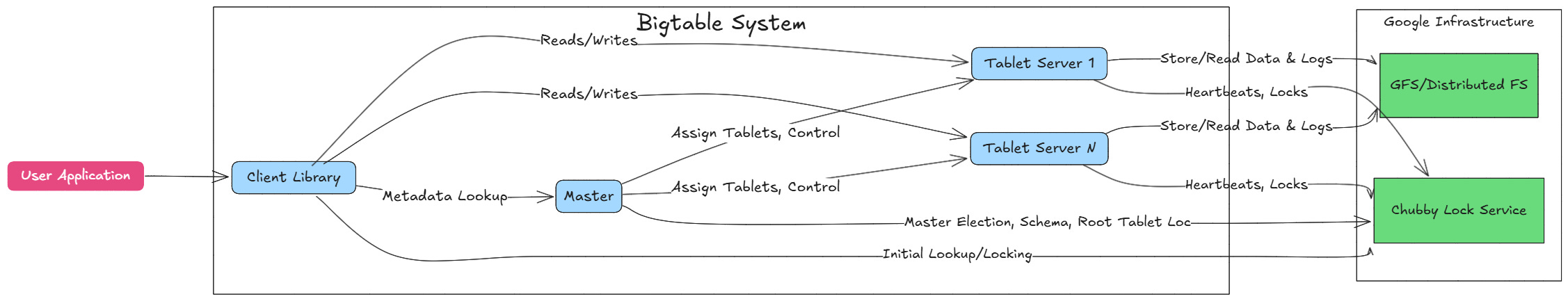
Okay, we have the data model. The paper outlines three major components:

1. Client Library: This is the code that applications link against to interact with Bigtable. It handles things like finding the right tablet server for a given row key, routing read/write requests, maybe doing some client-side buffering or caching, and handling retries. It hides much of the system's complexity from the application developer.

2. Master Server: There's typically one active master. Its job is primarily metadata management. It doesn't serve data reads or writes directly (this is key for scalability – the master isn't a bottleneck for common operations). What does it do?

   • Assigns tablets to tablet servers.

   • Detects the addition or expiration/failure of tablet servers.

   • Balances tablet server load (e.g., moving tablets around if one server gets too busy).

   • Handles schema changes (like creating or deleting tables and column families).

   • Garbage collection of obsolete files in GFS.

3. Tablet Servers: These are the workhorses. Each tablet server manages a set of tablets (typically 10-1000 tablets per server, according to the paper). For the tablets it manages, a tablet server:

   • Handles read and write requests from clients.

   • Split tablets that grow too large. When a tablet exceeds a configured size limit (e.g., 100-200 MB), the tablet server splits it into two roughly equal halves and informs the master.

   • Manages the storage and compaction of data for its tablets (we'll get into this!).

Underlying Infrastructure: Bigtable relies heavily on other pieces of Google's infrastructure:

• Google File System (GFS) or similar: Used to store the actual data files (SSTables) and commit logs in a persistent and replicated way. Bigtable leverages GFS for durability and availability of the underlying data.

• Chubby Distributed Lock Service: This is crucial for coordination. Bigtable uses Chubby for several critical tasks:

  • Ensuring there's only one active master at any time.

  • Storing the location of the root tablet (we'll explain this).

  • Discovering tablet servers and finalizing tablet server deaths.

  • Storing Bigtable schema information (column family details).

  • Storing access control lists.

Let's visualize this basic architecture.

High-Level Design of the Big Table System

Key Mechanism: Finding Data - Tablet Location

So, a client has a row key and wants to read or write data. How does it find the right tablet server holding the tablet for that row? Bigtable uses a clever, three-level hierarchy, somewhat analogous to B+ trees, to store tablet location information.

1. Level 1: The Root Tablet Location in Chubby: There's a file in Chubby that contains the location (i.e., the address of the tablet server currently serving it) of the root tablet. This location is well-known and cached by clients. If the client's cache is stale or the root tablet moves (which is rare), the client re-reads this file from Chubby.

2. Level 2: The Root Tablet: The root tablet itself is just like any other Bigtable tablet, except it never splits. It contains the location information for all tablets in a special METADATA table. Each entry in the root tablet maps a row key (representing the end row key of a METADATA tablet) to the location of that METADATA tablet.

3. Level 3: The METADATA Table: This table stores the location of all the user tablets. Each row in the METADATA table corresponds to a user tablet. The row key for a METADATA row is constructed from the table identifier and the end row key of the user tablet it describes. The values in that row contain the location (tablet server address) of the corresponding user tablet. The METADATA table can grow large, so it's split into multiple tablets itself, just like user tables.

Putting it Together (Client Lookup):

Let's say a client wants to access data for row key com.google.maps/us/ca/sanfrancisco.

1. The client library checks its cache for the location of the tablet serving this row range. Assume it's not cached or the cache seems stale.

2. The client asks Chubby for the location of the root tablet.

3. The client contacts the server holding the root tablet and asks: "Where can I find the METADATA tablet responsible for row keys around my_table_id + com.google.maps/us/ca/sanfrancisco?" The root tablet responds with the location of the relevant METADATA tablet.

4. The client contacts the server holding that METADATA tablet and asks: "Where can I find the user tablet responsible for row key com.google.maps/us/ca/sanfrancisco in my_table_id?" The METADATA tablet responds with the location of the specific user tablet server.

5. The client contacts the identified user's tablet server and performs the read or write operation.

Caching is Key: The client library caches these locations. Reads/writes usually only involve step 5. Steps 1-4 only happen on a cache miss or if the cached location turns out to be wrong (e.g., because a tablet was reassigned by the master). The paper notes, "In practice... clients require almost no communication with the master," and "clients typically make fewer than six RPCs per operation," even with uncached location information, often just one RPC when cached. This hierarchy ensures that finding data is scalable.

Here's a simplified diagram of the lookup:

Reads and Writes Work (Inside a Tablet Server)

Okay, the client found the right tablet server. What happens when a write or read request arrives?

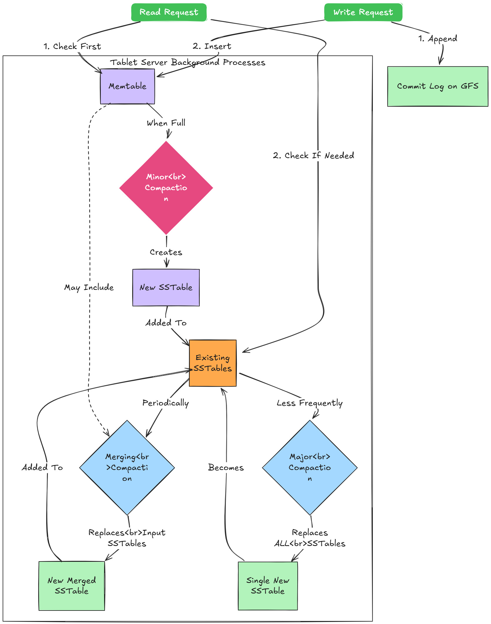
• Writes:

  1. Permission Check: The tablet server checks if the client has permission to write (using information likely retrieved from Chubby).

  2. Commit Log: The write is immediately appended to a commit log stored on the underlying distributed file system (GFS). This log ensures durability – if the tablet server crashes before the data is permanently stored, the log can be replayed on recovery.

  3. Memtable: After logging, the write is inserted into an in-memory sorted buffer called the memtable. The memtable keeps recent writes sorted by key, just like the overall Bigtable data model. It's typically implemented using something efficient for concurrent reads/writes and scans, like a skip list.

  That's it for the client's perspective – once the write is logged and in the memtable, it's considered done.

• Reads:

  1. Permission Check: Similar to writes, check permissions.

  2. Merged View: A read operation needs to consult both the in-memory memtable (which has the most recent updates) and the on-disk data structures (SSTables, see below) for that tablet. The tablet server creates a merged view of these two sources, respecting timestamps (newer values override older ones) and handling deletions (which are marked by special tombstone entries).

  3. Memtable First: The read checks the sorted memtable for the requested row/column(s).

  4. SSTables: If data isn't found in the memtable (or if older versions are needed), the server consults a sequence of immutable, on-disk files called SSTables (Sorted String Tables). These are stored in GFS.

SSTables: The On-Disk Reality

The memtable is in memory, so it's fast but has limited capacity and isn't persistent across crashes (that's what the commit log is for). As the memtable fills up, the tablet server needs to flush its contents to persistent storage. This process creates an SSTable.

• Immutable: Once an SSTable is written to GFS, it's never modified. This immutability greatly simplifies things:

  • No locking needed for concurrent reads.

  • Easy caching.

  • Simplifies recovery (no partial writes to worry about).

  • Deleted data isn't removed immediately; it's just marked with a tombstone or superseded by newer versions in the memtable or newer SSTables. Space is reclaimed later during compactions.

• Sorted: Like the memtable, an SSTable contains key-value pairs sorted lexicographically by key (row, column, timestamp). This allows for efficient lookups and scans.

• Structure: An SSTable typically consists of a sequence of data blocks, followed by an index block. The index block helps quickly locate the data block containing a specific key range without scanning the whole file. The index might be loaded into memory by the tablet server.

• Bloom Filters: To speed up reads, especially for non-existent rows or columns, SSTables can include Bloom filters. A Bloom filter is a probabilistic data structure that can quickly tell you if an element is definitely not in a set, or maybe is in the set. Before accessing an SSTable on GFS (which might involve network latency), the tablet server can check the Bloom filter (often loaded in memory). If the filter says the row/column doesn't exist, the SSTable access can be skipped entirely. This significantly helps performance for sparse datasets or random lookups.

Compactions: Keeping Things Tidy and Efficient

Over time, as writes happen and memtables are flushed, a tablet accumulates multiple SSTables. Reads might need to consult the memtable and all these SSTables to find the latest data and handle deletions. This can slow down reads. Also, deleted or overwritten data still consumes space in older SSTables.

To manage this, tablet servers periodically perform compactions:

1. Minor Compaction: When the memtable fills up, it's frozen, a new one is created, and the frozen memtable's contents are written out as a new SSTable to GFS. This is the primary way data moves from memory to disk. The commit log entries corresponding to the flushed memtable can then be discarded. This primarily reduces memory usage and recovery time (shorter log replay needed).

2. Merging Compaction: Periodically, the tablet server reads a few SSTables and the memtable, merges them together (applying updates, removing deleted/superseded data), and writes out a new SSTable containing the combined, sorted data. The input SSTables and memtable snapshot used for the merge are then discarded. This reduces the number of SSTables that need to be consulted during reads.

3. Major Compaction: This is a merging compaction that rewrites all SSTables for a tablet into a single, new SSTable. Crucially, this is the only process that fully reclaims the space used by deleted or overwritten data (because the original SSTables containing the old data are discarded). All deletion tombstones are also garbage collected during a major compaction. These are essential for reclaiming disk space but can be I/O intensive, so they are scheduled carefully.

Compactions happen in the background without interrupting ongoing reads and writes to the tablet.

Let's visualize the write path and compactions:

Refinements and Optimizations

The paper also discusses several important refinements that make Bigtable practical:

• Locality Groups: Column families can be grouped into "locality groups." Each locality group for a tablet is stored in its own set of SSTables. This allows for tuning performance. For example, you might put frequently accessed metadata columns in one locality group (possibly kept in memory) and the large page contents in another (likely on disk, maybe with different compression). Segregating access patterns like this can significantly improve read performance for common queries. If an application only reads columns from one family (e.g., metadata:), the system might only need to access the SSTables for that locality group.

• Compression: SSTables blocks can be compressed to save space on GFS and potentially improve read throughput (by reading less data from disk/network). The paper mentions using Bentley and McIlroy's scheme and Zippy. Compression can be configured per locality group.

• Caching: Tablet servers use two levels of caching:

  • Scan Cache: Caches key-value pairs returned by SSTable reads. Useful for workloads that read the same data repeatedly.

  • Block Cache: Caches entire SSTable blocks read from GFS. Useful for workloads with temporal locality (reading nearby rows/columns soon after).

• Bloom Filters: As mentioned before, these dramatically reduce the disk/network accesses needed for random reads, especially when checking for things that don't exist.

• Commit Log Implementation: To avoid GFS bottlenecks with many concurrent writes to the same log file, each tablet server actually writes its commit log to multiple log files, potentially multiplexing writes from different tablets across these files. This improves write throughput. Recovery involves sorting log entries by key (table, row, log sequence number) to handle potential duplicate entries if a server died mid-write.

• Tablet Splitting: When a tablet gets too large, the tablet server simply splits it along a row key boundary. It doesn't need to create new SSTables immediately; the new child tablets initially just share the parent's SSTables but only process requests for their respective halves of the row range. The master is notified of the split so it can update the METADATA table.

• Master Operations: The master monitors tablet servers via Chubby's lock mechanism and heartbeating. If a server loses its lock or stops heartbeating, the master assumes it's dead and reassigns its tablets to other live servers. Tablet recovery involves reading metadata, replaying the commit log from GFS for writes that weren't yet flushed to SSTables, and then making the tablet available for serving. Schema changes (like adding a column family) are initiated by the master and propagated lazily.

API and Usage

The Bigtable API described is relatively simple, focusing on the core data manipulation needs:

• Creating/deleting tables and column families (usually admin operations).

• Modifying cluster, table, or column family metadata (e.g., access control rights).

• Writing or deleting values.

• Reading values (looking up specific cells or scanning over row ranges).

• Single-row transactions: Bigtable supports atomic Read-Modify-Write sequences on data within a single row key. This allows clients to perform operations like atomically incrementing a counter or appending data to a cell value without external locking. This is a very useful feature for certain applications like hit counters.

Note that Bigtable does not support general, multi-row transactions like relational databases. Consistency is guaranteed only at the row level for these read-modify-write operations.

Lessons and Impact

So, what made Bigtable so important?

1. Demonstrated Scalability: It showed that you could build a highly scalable, available, and performant storage system for structured/semi-structured data on commodity hardware.

2. Flexible Data Model: The sparse, multidimensional map model with column families proved very effective for many large-scale applications where relational schemas were too rigid or inefficient.

3. Influence: Bigtable, along with GFS and MapReduce (described in other Google papers around the same time), laid the groundwork for many subsequent NoSQL databases and large-scale data processing systems. Concepts like column families, SSTables, memtables, compactions, and leveraging distributed file systems and lock services became common patterns in systems like HBase, Cassandra, LevelDB, and RocksDB.

4. Engineering Pragmatism: The paper highlights practical engineering choices: relying on robust underlying services (GFS, Chubby), making SSTables immutable, using Bloom filters, careful log management, and focusing master responsibilities on metadata to avoid bottlenecks.

It wasn't a perfect system for all problems – the lack of multi-row transactions, the reliance on specific infrastructure (Chubby/GFS), and the potential complexity of choosing good row keys are trade-offs. But for the target problems – massive scale, flexible schema, high throughput – it was a groundbreaking solution.

Wrapping Up

Going through the Bigtable paper feels like dissecting a masterclass in distributed systems engineering. They faced a hard challenge – data scale beyond what existing tools could handle efficiently – and architected a solution by combining several clever ideas: the flexible data model, the tablet-based partitioning, the three-level location hierarchy, the write-ahead log + memtable + immutable SSTable design, background compactions, and leveraging foundational services like GFS and Chubby. Each piece plays a critical role in achieving the overall goals of scalability, performance, and availability. It’s a system designed with a deep understanding of the trade-offs involved in building large-scale distributed systems on commodity hardware. Understanding Bigtable gives you a fantastic foundation for understanding many of the NoSQL and distributed database technologies that followed.

Share for Good Karma 😇

Liked this article? Make sure to ❤️ click the like button.

Feedback or addition? Make sure to 💬 comment.

Know someone who would find this helpful? Make sure to 🔁 share this post.

Your support means a great deal!

Thank you! Let’s learn together!