
Paper I read this week : MapReduce
Each week, I’ll break down a research paper I’ve read, sharing the coolest bits and what I learned in a quick summary."

🚀🚀Welcome to our weekly roundup where we unpack fascinating ideas from the latest research papers I’ve explored!
Expect concise summaries, key takeaways, and visual breakdowns—like flowcharts of complex systems to make cutting-edge concepts accessible.
Whether you’re a tech enthusiast, researcher, or curious learner, this section will spark insights and keep you at the forefront of innovation. Dive in and let’s explore together! 🚀🚀
I have started summarizing all the paper I have read in the past and in future (If you have any paper as suggestion feel free to tag me in the comments. Hope you enjoy!
You can read the paper here:
This paper is just amazing, authored by Jeffrey Dean and Sanjay Ghemawat at Google.
Introduction
Imagine you're faced with a mountain. Not just any mountain, but a mountain made of information.
Think about Google – they have copies of huge chunks of the internet, logs of every search query, tons of data.
We're talking terabytes, petabytes – numbers so big they almost lose meaning!
Now, imagine you need to find something specific in that mountain, or count something across all of it, like how many times the word "aardvark" appears on every webpage ever indexed.
How would you even begin to tackle that?
Doing it on one computer?
Forget it!
It would take years, centuries maybe!
Even a super-duper powerful computer would choke on that much data.
So, what do you do?
Well, what if you had, say, a thousand computers? Or ten thousand?
Not fancy supercomputers, just regular, cheap, commodity PCs – the kind that might break down occasionally.
Could you use them? That's the problem Google faced.
They had this massive cluster of machines, this sea of data. They needed a simple way for their smart engineers to write programs that could process all that data, spread across all those machines, without getting bogged down in the messy details of how to split the work, send it out, handle machines failing, and collect the results.
That’s where this brilliant idea called MapReduce comes in. It’s a programming model – a way of thinking about the problem – and a system that handles all the grungy background work. It's beautiful because it takes a potentially terrifyingly complex problem and breaks it down into something manageable, something elegant.
Think of it like this: You have a massive pile of surveys, maybe millions of them, from a giant census. You want to find out the average age of people in each city. How would you do it with an army of helpers?
You wouldn't give the whole pile to one person! You'd probably do something like this:
Divide the Pile: Split the huge pile of surveys into smaller stacks, maybe one stack for each helper.
First Pass (Map): Tell each helper, "Go through your stack. For each survey, write down the City and the Age on a separate little note card." So, each helper generates a bunch of (City, Age) note cards. This is the MAP step. Each helper is working independently on their chunk of data.
Collect and Sort (Shuffle): Now you have thousands of these little note cards from all the helpers. You need to get all the cards for the same city together. So, you collect all the cards and sort them by city. All the "New York" cards go in one pile, all the "London" cards in another, and so on. This crucial sorting and grouping step is the SHUFFLE (or Shuffle and Sort).
Second Pass (Reduce): Now, assign different helpers (or maybe the same ones, re-tasked) to each city pile. Tell the helper in charge of the "New York" pile: "Take all these cards. Add up all the ages and count how many cards you have. Calculate the average age for New York." Do the same for London, Tokyo, etc. This is the REDUCE step. Each helper takes a group of values associated with a single key (the city) and produces a single output (the average age).
Final Output: Collect the results from each "Reduce" helper, and you have your final answer: the average age for each city.
See?
You broke the giant task into smaller, identical tasks (Map), shuffled the intermediate results, and then did another set of smaller, identical tasks (Reduce) to get the final answer. The beauty is that the Map helpers don't need to talk to each other, and the Reduce helpers (mostly) don't need to talk to each other. This makes it easy to spread the work across many, many machines.
The MapReduce paper from Google said: "Hey, we do this kind of data processing all the time. Let's build a general-purpose system that handles this pattern. Programmers just need to provide the logic for Step 2 (the Map function) and Step 4 (the Reduce function), and our system will handle everything else: splitting the data, running the tasks on hundreds or thousands of machines, sorting the intermediate data, and dealing with machines that inevitably crash!"
Isn't that neat? It simplifies the problem for the programmer down to its core logic. They focus on what to compute, not how to distribute it and make it reliable.
Let's dive deeper into how this magic actually happens inside the system.
The Core Programming Model: Map and Reduce Functions
Alright, let's get a bit more precise, like physicists like to be! The programmer using MapReduce provides two key pieces of code:
The map function:
Input: It takes a key/value pair. What this pair represents depends on the input data. For our census example, the input might be (document_id, survey_text). For processing web logs, it might be (line_number, log_entry_text).
Output: It produces a list of intermediate key/value pairs. In our census example, the map function reads the survey text, finds the city and age, and outputs (City, Age). So, one input pair might generate zero, one, or multiple output pairs. For a Word Count example, the input could be (document_id, document_text). The map function would read the text, split it into words, and for each word, output (word, 1). So the word "the" appearing 3 times would result in three outputs: ("the", 1), ("the", 1), ("the", 1).
The reduce function:
Input: It takes an intermediate key and a list of all intermediate values associated with that key. The MapReduce framework guarantees that all values for the same key are brought together to a single reduce call. In the census example, a reduce call would get ("New York", [25, 30, 45, 22, ...]). For Word Count, it would get ("the", [1, 1, 1, 1, ...]).
Output: It produces a list of final output values (often just one value, or perhaps final key/value pairs). For the census, the reduce function calculates the average of the input list of ages and outputs ("New York", average_age). For Word Count, it sums the list of 1s and outputs ("the", total_count).
The programmer writes these two functions, often just a few lines of code each. They don't worry about parallelism, data distribution, or failures. That's the framework's job.
How the MapReduce System Executes a Job
Now, let's peek under the hood. How does the system take these simple map and reduce functions and run them on a giant cluster? It's like a well-orchestrated dance, managed by a Master node and performed by many Worker nodes.
Imagine the Master as the conductor and site foreman, and the Workers as the orchestra musicians or construction crew.
Here's the sequence of events:
Input Splitting: The system first takes the massive input data (sitting on a distributed file system, like Google File System - GFS) and splits it into many smaller chunks, typically 16MB to 64MB each. Let's say we have 10 Terabytes of data, we might split it into hundreds of thousands of chunks.
Job Submission: The user submits the MapReduce job to the Master node. This includes the code for map and reduce, the location of the input data, and where to put the final output.
Master Assigns Map Tasks: The Master identifies idle Worker nodes. For each input split, it assigns a Map task to a Worker. Ideally, the Master tries to assign the task to a worker machine that already has a copy of that input split stored locally (or is physically close in the network rack). This is locality optimization – it saves precious network bandwidth, like reading a book that's already on your desk instead of fetching it from the library basement.
Workers Execute Map Tasks: The assigned Worker reads the input split assigned to it. It parses the key/value pairs from the input data. For each pair, it calls the user's map function. The intermediate key/value pairs produced by map are buffered in the Worker's memory.
Intermediate Data Partitioning & Storage: Periodically, the Worker writes these buffered intermediate pairs to its local disk. Crucially, it partitions these pairs based on the intermediate key. It uses a partitioning function (often something simple like hash(key) mod R, where R is the number of Reduce tasks) to decide which of the R partitions this key belongs to. Think of this as sorting the note cards into R different bins locally before sending them off. The locations of these buffered files on local disk are reported back to the Master.
Master Assigns Reduce Tasks: Once the Master sees that Map tasks are completing and reporting the locations of their intermediate data, it starts assigning Reduce tasks to idle Workers. Each Reduce task is responsible for one of the R output partitions.
Workers Execute Reduce Tasks (The Shuffle): The Worker assigned a Reduce task (say, partition #3) gets the locations of all the relevant intermediate data (the contents of bin #3) from the Master. It then uses remote procedure calls (RPCs) to pull this data from the local disks of all the Map workers that generated data for partition #3. This phase of fetching the data is the Shuffle.
Sorting: As the Reduce worker receives the intermediate data, it sorts it by the intermediate keys. Why? So that all occurrences of the same key are grouped together. If multiple Map tasks emitted ("the", 1), the Reduce worker needs all those 1s together to process them. This sort is often done automatically as data arrives and merged.
Calling the Reduce Function: The Reduce worker iterates through the sorted intermediate data. For each unique intermediate key, it gathers the key and the corresponding list of values (key, [value1, value2, ...]) and calls the user's reduce function.
Writing Final Output: The output of the reduce function is appended to a final output file for this reduce partition, typically stored back onto the distributed file system (GFS).
Job Completion: When all Map and Reduce tasks have completed successfully, the Master wakes up the user program. The output of the MapReduce job is now available in the R output files (or sometimes combined into one, depending on configuration).
Phew! That's the flow. Notice how the data moves: from the distributed file system to Map workers, then intermediate data to Map workers' local disks, then shuffled across the network to Reduce workers, processed, and finally written back to the distributed file system.
Let's visualize some of these steps with diagrams.
Diagram 1: Overall MapReduce Flow

See? It's like an assembly line. Raw materials (Input Data) go in, get processed in parallel by the first set of workers (Map Phase), the partially finished goods are sorted and grouped (Intermediate Data, Shuffle & Sort), then processed by a second set of workers (Reduce Phase), and finally, the finished products (Output Data) emerge. The key is the parallelism at the Map and Reduce stages and that clever Shuffle step in the middle.
The Master and the Workers: Keeping Things Running
The Master is the brain of the operation. It doesn't do the heavy lifting of data processing, but it coordinates everything. What does it need to keep track of?
Task Status: For every Map task and every Reduce task, the Master knows whether it's idle (waiting to be assigned), in-progress (running on a worker), or completed.
Worker Status: It knows which workers are available.
Intermediate File Locations: Crucially, for completed Map tasks, the Master knows where on the Map workers' local disks the R intermediate files are stored. This information is needed to tell the Reduce workers where to fetch their data from.
Diagram 2: Master-Worker Interaction
The Master is like the foreman on a construction site. It gets the blueprints (the user's job), tells the workers (Worker A, Worker B) what specific jobs to do ("You lay bricks for this section," "You pour concrete there"). The workers periodically check in ("Yep, still working!"). When a worker finishes a stage, they report back ("Bricklaying for section 1 done! Here's where the pipes need to connect"). The foreman notes this down and assigns the next stage ("Okay, Plumber, connect the pipes based on where the Bricklayer left off"). It keeps track of everything until the whole building is finished.
The Crucial Shuffle and Sort
This middle phase is really where a lot of the magic connects the Map output to the Reduce input. Let's zoom in.
After a Map worker finishes its task, it has produced R files on its local disk, one for each reducer partition, decided by the partitioning function hash(intermediate_key) mod R.
When a Reduce worker starts, say for partition j, it needs to get the j-th file from every Map worker.
Diagram 3: The Shuffle & Sort Phase (Focus on one Reduce Task)
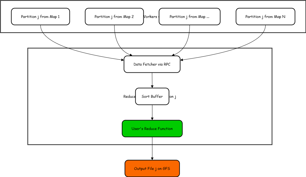
Imagine after the first step (Map), each helper put their note cards into R separate bins on their own desk. Now, helper Jane is responsible for consolidating all the "New York" information (let's say New York corresponds to bin #3, our partition j). Jane needs to go to every other helper's desk and grab only the cards from their bin #3. She brings all those bin #3 cards back to her desk (that's the Shuffle/Fetch). Then, before she can calculate the average age, she first arranges all the cards alphabetically by person's name, maybe, or just groups all the ages together (that's the Sort). Then she can finally run through the grouped ages and calculate the average (that's the Reduce function).
Handling Failure
This is where MapReduce truly shines compared to trying to build such a system yourself. Remember, we're using thousands of cheap machines. They will fail! Disks break, machines crash, networks hiccup. If your whole calculation stops every time one machine out of 2000 has a problem, you'll never finish anything!
MapReduce is designed for this from the ground up.
Worker Failure:
The Master periodically pings each Worker (sends a little "Are you there?" message). If a Worker doesn't respond after a certain time, the Master marks it as failed. Now, what happens to the tasks that the worker was running?
If it were an in-progress Map task: The Master resets its status to idle and schedules it on another available Worker. The work is simply redone. This is okay because Map tasks are designed to be idempotent based on their input split – running it again produces the same intermediate output (or should!).
If it was a completed Map task: This is a bit trickier because its intermediate output (stored on its local disk) is now lost! So, the Master must reschedule this Map task to another worker. Why? Because that intermediate data is needed by potentially all the Reduce tasks.
If it was an in-progress Reduce task: The Master resets its status to idle and reschedules it on another worker. The new worker will re-fetch the intermediate data (which is still available from the completed Map tasks) and redo the Reduce work. The final output for that partition will be overwritten or managed by the distributed file system as Task)
Diagram 4: Worker Failure Handling

Think of the foreman again. He sends worker Joe to lay bricks. He checks in, "Joe, how's it going?" No answer. Checks again. Still nothing. Foreman says, "Okay, Joe must have gone home sick (crashed!). That section of wall he was working on might be half-finished and useless." He tells another worker, Mary, "Mary, I need you to go lay the bricks for that same section Joe was doing. Start from scratch for that section." If Joe had finished his section but stored some crucial measurements on a notepad he took with him when he got sick, the foreman would still need Mary to redo Joe's entire section to regenerate those measurements! If Joe was calculating a final summary (Reduce task) and got sick, the foreman just tells Mary, "Go redo that summary calculation."
Master Failure:
This is much less common, but what if the Master itself fails? That sounds catastrophic! The original paper mentions a simple solution: the Master periodically writes checkpoints of its state (task statuses, worker statuses, intermediate file locations) to the distributed file system. If the Master process dies, a new one can be started, read the latest checkpoint, and resume coordinating the job from where the old one left off. More sophisticated systems might use replication or leader election, but the core idea is recovery through saved state.
Diagram 5: Master Failure
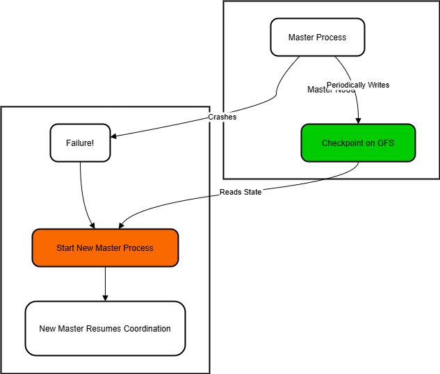
What if the foreman gets sick? Disaster? Not quite. Imagine the foreman keeps a very detailed logbook (the checkpoint) of exactly which worker is doing what, what's finished, and where all the materials are. He saves this logbook in a safe place (the distributed file system) every hour. If the foreman suddenly vanishes, the construction company can quickly bring in a new foreman. The new foreman finds the logbook, reads the last entry, and says, "Okay, I see Joe finished section A, Mary is working on section B... let's pick up right where we left off!" They might lose a tiny bit of coordination time, but the whole project doesn't have to restart from zero.
Refinements and Clever Tricks
The basic MapReduce model is powerful, but the Google paper describes several refinements that make it even more efficient or flexible.
Locality Optimization:
We touched on this. The distributed file system (GFS) often stores chunks of a file replicated on multiple machines (usually 3). When the Master assigns a Map task for input split X, it knows which machines hold replicas of X. It tries its best to schedule the Map task on one of those machines. If not possible (e.g., all those machines are busy), it tries to pick a worker on the same network rack as a machine holding the data. This minimizes network traffic for reading the initial input. Fetching data across the network is way slower than reading from a local disk!
Diagram 6: Locality Optimization

This is just common sense, right? If you need to read a chapter from a huge encyclopedia, and you know there's a copy on the desk right next to you (Worker X), you read that one! If that desk is occupied, but there's another copy on a desk in the same room (Worker Y on the same rack), you walk over there – it's pretty quick. Only if both are unavailable would you go down to the library archives three floors down (Worker Z on a different rack) – that takes much longer! The Master tries the fastest option first.
Task Granularity:
How many Map tasks (M) and Reduce tasks (R) should there be?
M (Map tasks): You want many more Map tasks than there are worker machines in your cluster. Why? Load balancing. If you have 1000 workers and only 1000 tasks, and one task takes much longer than others, many workers might sit idle near the end. If you have, say, 200,000 Map tasks for 1000 workers, each worker gets assigned many small tasks. When a worker finishes a task, it grabs another. This keeps all workers busy and helps mitigate the impact of slow machines or unlucky task assignments. The Master only needs to keep track of about M + R task statuses, which is manageable.
R (Reduce tasks): The number of Reduce tasks is often specified by the user. It determines the number of output files. Having too few Reduce tasks can create a bottleneck in the final phase. Having too many might increase the overhead of the shuffle phase and result in very small output files. It's a tuning parameter.
Backup Tasks
Sometimes, a machine isn't dead, just slow. Maybe it has a bad disk, or other processes are hogging its CPU. This one slow worker (a "straggler") performing the very last Map or Reduce task can delay the completion of the entire job significantly!
MapReduce has a clever trick: Near the end of the Map phase (or Reduce phase), the Master identifies any remaining in-progress tasks that are taking much longer than average. For each such straggler task, it schedules a backup execution of the same task on another idle worker. The task is considered complete whenever either the original execution or the backup execution finishes first. The other one is then killed. This significantly reduces the job completion time in the presence of slow machines.
Diagram 7: Backup Tasks (Stragglers)

Imagine one worker, "Slowpoke Steve," is taking forever on his little piece of the job, and everyone else is finished and waiting. The foreman notices Steve lagging. He doesn't just wait! He tells another idle worker, "Fast Fiona," "Hey, can you do Steve's task too? Just in case?" Now Steve and Fiona are racing. Whoever finishes first, the foreman takes their result and tells the other one, "Okay, you can stop now, we got it." This way, one slowpoke doesn't hold up the entire project! It costs a little extra computation, but it saves a lot of waiting time.
Combiner Function
This is a neat optimization, especially for jobs like Word Count. Remember the Map output for Word Count is (word, 1) for every single word? If a document contains "the" 100 times, the Map task emits ("the", 1) one hundred times. All these identical pairs have to be written to the local disk, sent over the network during the shuffle, and sorted by the Reducer. That's a lot of data!
The user can optionally provide a Combiner function. This function runs on the Map worker after the Map function completes, but before the output is written to local disk for the shuffle. The Combiner function typically has the same code as the Reduce function.
In the Word Count example, the Combiner would run on the Map worker. It would take all the ("the", 1) pairs generated by that single Map task, sum them up locally, and output a single pair: ("the", 100). This significantly reduces the amount of data written locally and transferred during the shuffle. It's a form of local pre-aggregation.
Diagram 8: Combiner Function

Think of Word Count again. The Map helper is making little note cards: "the, 1", "the, 1", "the, 1"... maybe hundreds for just one document! Before sending these off to the sorting area, the helper notices, "Hey, I've got a huge stack of 'the, 1' cards just from my own work!" The Combiner is like telling the helper: "Before you put those cards in the bins to be shuffled, just count up how many 'the, 1' cards you made, and replace that whole stack with a single card saying 'the, 100'." This helper does this for all words they processed. Now, instead of sending hundreds of tiny cards, they send just a few summary cards. Much less paper to move around! It only works if the operation (like summing counts) can be done partially like this.
Partitioning Function
We mentioned that intermediate data is partitioned using hash(key) mod R. Users can replace this default partitioning function. Why? Maybe they want to ensure that all keys related to a specific domain name (e.g., all URLs from *.google.com) end up in the same output file. They could provide a custom partition function that looks at the key (the URL) and assigns partitions based on the domain, ensuring related keys go to the same Reducer.
Diagram 9: Partitioning Function

Usually, the system just randomly assigns intermediate results to Reducers (using the hash function). But maybe you want all the information about California to go to Reducer #1, all about Texas to Reducer #2, etc. The custom partitioning function is like telling the sorting helpers: "Don't just put these cards into bins randomly based on the last letter of the city name. Instead, look at the state mentioned on the card, and put all California cards in Bin 1, all Texas cards in Bin 2..." This gives the user control over which keys end up being processed together and in which final output file.
Other Refinements:
Input/Output Types: The paper mentions support for different data formats, not just text lines. Users could provide reader/writer interfaces for binary formats, database inputs, etc.
Skipping Bad Records: Sometimes, user code might crash on certain input records due to bugs or corrupted data. The framework can detect this, skip the bad record, and continue processing, rather than failing the entire task. It keeps track of skipped records so the user can investigate later.
Counters: The framework provides a counter facility. User code (Map or Reduce) can increment named counters (e.g., "Words starting with 'Q'", "Corrupt log entries found"). The Master aggregates these counts from all workers, providing useful statistics about the job's execution.
Local Execution: For debugging, there's a library implementation that runs the entire MapReduce process locally on a single machine, making it easier to test the user's Map and Reduce functions.
Use Cases: What's it Good For?
The paper lists several real-world applications at Google where MapReduce was incredibly useful:
Distributed Grep: Searching for a pattern across petabytes of data. The Map function emits a line if it matches the pattern. The Reduce function is just the identity function (copies the intermediate data to the output).
Reverse Web-Link Graph: Finding all pages that link to a given page. The Map function outputs (target_URL, source_URL) for each link found on a source page. The Reduce function concatenates the list of source URLs for a given target URL, outputting (target_URL, [list_of_source_URLs]).
Inverted Index: This is fundamental to search engines. Creating an index mapping words to the documents they appear in. The Map function parses documents and outputs (word, document_ID). The Reduce function collects all document IDs for a given word and outputs (word, [list_of_document_IDs]).
Distributed Sort: Sorting a massive dataset. This uses a clever MapReduce approach where the Map function extracts the sort key and outputs (key, record). The framework's shuffle/sort mechanism does most of the heavy lifting! A simple Reduce function (identity) just writes the already sorted data to the output files. The partitioning function is crucial here to define the ranges of keys for each output file.
Key Takeaways: Why Was MapReduce Such a Big Deal?
Alright, let's sum this up. Why did this idea catch on like wildfire, not just at Google but across the industry (leading to things like Apache Hadoop)?
Simplicity: Programmers write simple Map and Reduce functions. They don't need to be experts in distributed systems, network programming, or fault tolerance. This massively broadened the pool of engineers who could process huge datasets.
Scalability: It runs on large clusters of commodity machines. Need more processing power? Just add more machines! The framework handles the distribution.
Fault Tolerance: It automatically handles machine failures, which are common in large clusters. Jobs can actually finish reliably.
Efficiency: Techniques like locality optimization and combiners make it perform well in practice. Backup tasks handle stragglers.
Generality: The model is surprisingly flexible and applies to a wide range of problems involving large-scale data analysis.
It wasn't necessarily the fastest possible way to solve any single one of these problems if you were willing to write highly specialized, complex distributed code. But it was incredibly good enough for a vast range of problems and dramatically easier to use, making large-scale data processing accessible.
Diagram 10: MapReduce - Key Benefits Summary

Conclusion
So, there you have it! MapReduce. It's not black magic, it's just a very clever way to organize work. You take a giant problem, you Map it into smaller, manageable pieces that can be done independently. You Shuffle the results around so the right pieces get together. Then you Reduce those pieces down to the final answer. The system underneath handles all the messy details of running this on potentially unreliable machines. It's a beautiful example of abstraction – hiding the complexity so smart people can focus on solving the actual problem. It fundamentally changed how we approach computation on massive datasets. Isn't that something? Any questions? Good! Now, let's think about how we could break this explanation... just kidding!
🌋MapReduce Limitations and Modern Alternatives🌋
While MapReduce was revolutionary, it has limitations in terms of speed and flexibility for iterative and complex data processing tasks. This is where tools like Apache Spark come in.
🎈Apache Spark
Spark leverages in-memory processing, meaning it keeps data in RAM for very fast calculations compared to MapReduce’s reliance on disk storage. It handles a wider range of tasks, including SQL queries, machine learning, and real-time data processing (streaming).
🎈Apache Flink
Apache Flink is another powerful framework used for real-time data processing (stream processing). It offers similar capabilities to Spark Streaming, allowing for immediate analysis of data as it arrives. This is a specialized tool for scenarios requiring real-time data analysis, often used alongside Spark for a complete big data processing toolkit.
🎈Hadoop
Hadoop is a broader ecosystem that provides the foundation for tools like Spark and MapReduce to run. It includes a distributed file system (HDFS) for storing large datasets across multiple machines and a resource management system (YARN) that allocates resources (CPU, memory) to applications like Spark or MapReduce.
Think of it as the underlying infrastructure that Spark and other tools use to manage and store big data.
🎈Cloud-based Services (AWS, Azure, GCP)
Cloud providers like AWS, Azure, and Google offer managed data processing solutions that often streamline the use of MapReduce frameworks. These include AWS EMR (which supports Hadoop), Azure HDInsight, and Google Cloud Dataflow (Google’s successor to classic MapReduce, built for both batch and streaming data).